Coaxial Waveguide¶

Cutoff frequency of PEC wavefuide¶

[1]:

import numpy as np
import matplotlib.pyplot as plt
from IPython.display import display
import pymwm
plt.style.use('seaborn-notebook')
plot_params = {
    'figure.dpi': 96,
    'axes.labelsize': 'xx-large',
    'xtick.labelsize': 'x-large',
    'ytick.labelsize': 'x-large',
    'legend.fontsize': 'large',
    'savefig.bbox': 'tight',
    'savefig.pad_inches': 0.03,
}
plt.rcParams.update(plot_params)

[2]:

import numpy as np
import scipy.special as sp
import numpy.testing as npt
import pymwm
from pymwm.cutoff import Cutoff

co = Cutoff(16, 8)

2022-03-07 18:32:29,521 INFO services.py:1374 -- View the Ray dashboard at http://127.0.0.1:8265

[3]:

co(('E', 1, 2), 0.5)

[3]:

6.5649423823227595

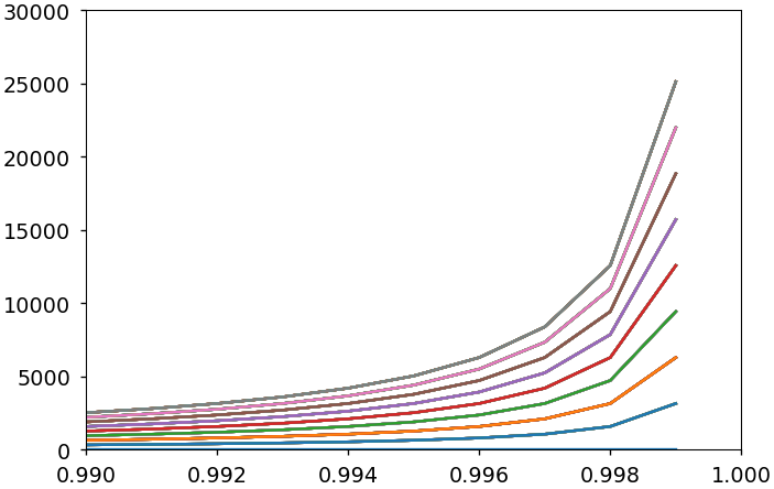
[4]:

import matplotlib.pyplot as plt
import numpy as np

fig = plt.figure(facecolor='white')

n = 0
for m in range(8):
    df = co.samples.query(f"pol == 'E' and n == {n} and m == {m + 1}")
    plt.plot(df['rr'], df['val'], label=f"E{n}{m + 1}")
# plt.legend(bbox_to_anchor=(1, 1), loc='upper left', borderaxespad=1, fontsize=7)

plt.xlim(0.99,1.0)
plt.ylim(0,30000)

#0.999まで有効

[4]:

(0.0, 30000.0)

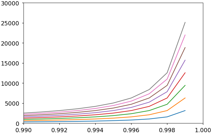
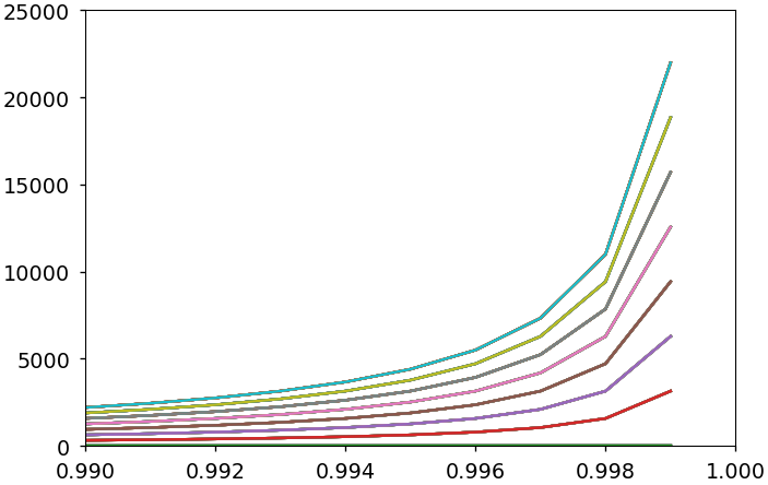
../_images/notebooks_03_coaxial_waveguide_5_1.png

[5]:

import matplotlib.pyplot as plt
import numpy as np

fig = plt.figure(facecolor='white')

for n in range(1, 16):
    for m in range(8):
        df = co.samples.query(f"pol == 'E' and n == {n} and m == {m + 1}")
        plt.plot(df['rr'], df['val'], label=f"E{n}{m + 1}")
# plt.legend(bbox_to_anchor=(1, 1), loc='upper left', borderaxespad=1, fontsize=7)

plt.xlim(0.99,1.0)
plt.ylim(0,25000)

#0.999まで有効

[5]:

(0.0, 25000.0)

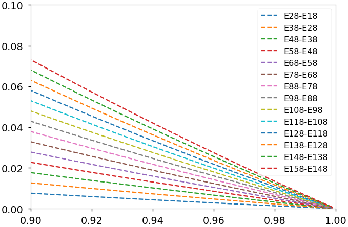
../_images/notebooks_03_coaxial_waveguide_6_1.png

[6]:

fig = plt.figure(facecolor='white')

for m in range(7, 8):
    for n in range(1, 15):
        df1 = co.samples.query(f"pol=='E' and n=={n} and m=={m+1}")
        df2 = co.samples.query(f"pol=='E' and n=={n+1} and m=={m+1}")
        val_dif = df2['val'].to_numpy() - df1['val'].to_numpy()
        plt.plot(df1['rr'], val_dif, "--", label=f"E{n+1}{m+1}-E{n}{m+1}")

plt.legend()

plt.xlim(0.9,1)
plt.ylim(0,0.1)

[6]:

(0.0, 0.1)

../_images/notebooks_03_coaxial_waveguide_7_1.png

[7]:

import matplotlib.pyplot as plt
import numpy as np

fig = plt.figure(facecolor='white')

for n in range(16):
    for m in range(8):
        df = co.samples.query(f"pol=='M' and n=={n} and m=={m+1}")
        plt.plot(df['rr'], df['val'], label=f"M{n}{m+1}")
# plt.legend(bbox_to_anchor=(1, 1), loc='upper left', borderaxespad=1, fontsize=7)

plt.xlim(0.99, 1)
plt.ylim(0,30000)

#0.999まで有効

[7]:

(0.0, 30000.0)

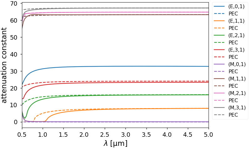
../_images/notebooks_03_coaxial_waveguide_8_1.png

Dispersion relation¶

[8]:

wl_max = 5.0
wl_min = 0.5
params: dict = {
    "core": {"shape": "coax", "r": 0.15, "ri": 0.1, "fill": {"RI": 1.0}},
    "clad": {"book": "Au", "page": "Stewart-DLF", "bound_check": False},
    "bounds": {"wl_max": wl_max, "wl_min": wl_min, "wl_imag": 100.0, "v_lim": False},
    "modes": {"num_n": 6, "num_m": 2},
}
wg1 = pymwm.create(params)
wg1.alpha_all

2022-03-07 18:33:28,725 INFO services.py:1374 -- View the Ray dashboard at http://127.0.0.1:8265
2022-03-07 18:33:46,317 INFO services.py:1374 -- View the Ray dashboard at http://127.0.0.1:8265
2022-03-07 18:34:03,944 INFO services.py:1374 -- View the Ray dashboard at http://127.0.0.1:8265
2022-03-07 18:34:21,723 INFO services.py:1374 -- View the Ray dashboard at http://127.0.0.1:8265
2022-03-07 18:34:40,724 INFO services.py:1374 -- View the Ray dashboard at http://127.0.0.1:8265

[8]:

[('E', 1, 1),
 ('E', 1, 2),
 ('E', 2, 1),
 ('E', 2, 2),
 ('E', 3, 1),
 ('E', 3, 2),
 ('E', 4, 1),
 ('E', 4, 2),
 ('E', 5, 1),
 ('E', 5, 2),
 ('M', 0, 1),
 ('M', 0, 2),
 ('M', 1, 1),
 ('M', 1, 2),
 ('M', 2, 1),
 ('M', 2, 2),
 ('M', 3, 1),
 ('M', 3, 2),
 ('M', 4, 1),
 ('M', 4, 2),
 ('M', 5, 1),
 ('M', 5, 2),
 ('E', 0, 1),
 ('E', 0, 2),
 ('E', 1, 1),
 ('E', 1, 2),
 ('E', 2, 1),
 ('E', 2, 2),
 ('E', 3, 1),
 ('E', 3, 2),
 ('E', 4, 1),
 ('E', 4, 2),
 ('E', 5, 1),
 ('E', 5, 2),
 ('M', 1, 1),
 ('M', 1, 2),
 ('M', 2, 1),
 ('M', 2, 2),
 ('M', 3, 1),
 ('M', 3, 2),
 ('M', 4, 1),
 ('M', 4, 2),
 ('M', 5, 1),
 ('M', 5, 2)]

[9]:

fig = plt.figure(facecolor='white')
wg1.plot_beta(('E', 0, 1), "-", wl_max=wl_max, wl_min=wl_min, comp='real')
wg1.plot_beta(('E', 1, 1), "-", wl_max=wl_max, wl_min=wl_min, comp='real')
wg1.plot_beta(('E', 2, 1), "-", wl_max=wl_max, wl_min=wl_min, comp='real')
wg1.plot_beta(('E', 3, 1), "-", wl_max=wl_max, wl_min=wl_min, comp='real')
wg1.plot_beta(('M', 0, 1), "-", wl_max=wl_max, wl_min=wl_min, comp='real')
wg1.plot_beta(('M', 1, 1), "-", wl_max=wl_max, wl_min=wl_min, comp='real')
wg1.plot_beta(('M', 2, 1), "-", wl_max=wl_max, wl_min=wl_min, comp='real')
wg1.plot_beta(('M', 3, 1), "-", wl_max=wl_max, wl_min=wl_min, comp='real')
plt.show()
fig = plt.figure(facecolor='white')
wg1.plot_beta(('E', 0, 1), "-", wl_max=wl_max, wl_min=wl_min, comp='imag')
wg1.plot_beta(('E', 1, 1), "-", wl_max=wl_max, wl_min=wl_min, comp='imag')
wg1.plot_beta(('E', 2, 1), "-", wl_max=wl_max, wl_min=wl_min, comp='imag')
wg1.plot_beta(('E', 3, 1), "-", wl_max=wl_max, wl_min=wl_min, comp='imag')
wg1.plot_beta(('M', 0, 1), "-", wl_max=wl_max, wl_min=wl_min, comp='imag')
wg1.plot_beta(('M', 1, 1), "-", wl_max=wl_max, wl_min=wl_min, comp='imag')
wg1.plot_beta(('M', 2, 1), "-", wl_max=wl_max, wl_min=wl_min, comp='imag')
wg1.plot_beta(('M', 3, 1), "-", wl_max=wl_max, wl_min=wl_min, comp='imag')
plt.show()

../_images/notebooks_03_coaxial_waveguide_11_0.png

../_images/notebooks_03_coaxial_waveguide_11_1.png

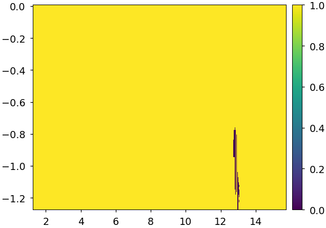
[10]:

wl_max = 5.0
wl_min = 0.5
params: dict = {
    "core": {"shape": "coax", "r": 0.15, "ri": 0.1, "fill": {"RI": 1.0}},
    "clad": {"book": "Au", "page": "Stewart-DLF", "bound_check": False},
    "bounds": {"wl_max": wl_max, "wl_min": wl_min, "wl_imag": 100.0},
    "modes": {"num_n": 6, "num_m": 2},
}
wg = pymwm.create(params)
betas, convs, samples = wg.betas_convs_samples(params)
samples.plot_convs(convs, ('E', 2, 1))

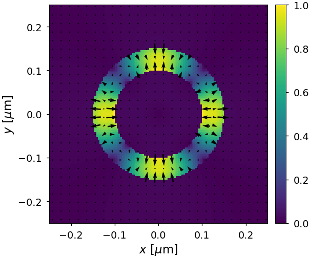
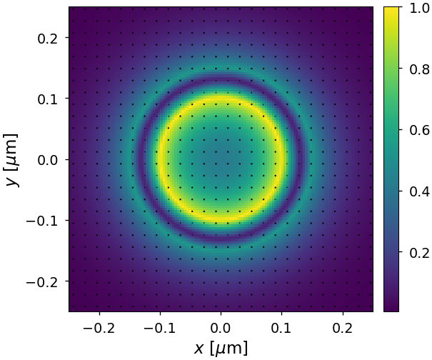
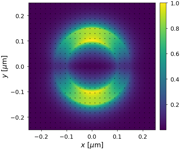
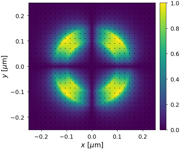
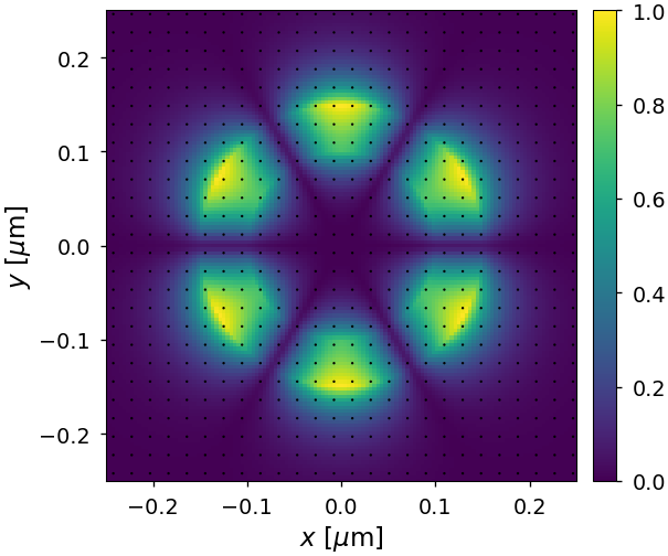
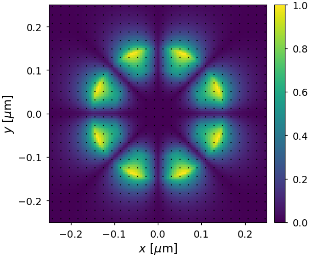
../_images/notebooks_03_coaxial_waveguide_12_0.png

[15]:

wl = 1.0
w = 2 * np.pi / wl
wg1.plot_e_field(w, dir='v', alpha=('E', 0, 1))
wg1.plot_e_field(w, dir='h', alpha=('E', 1, 1))
wg1.plot_e_field(w, dir='h', alpha=('E', 2, 1))
wg1.plot_e_field(w, dir='h', alpha=('E', 3, 1))
wg1.plot_e_field(w, dir='h', alpha=('E', 4, 1))
wg1.plot_e_field(w, dir='h', alpha=('M', 0, 1))
wg1.plot_e_field(w, dir='h', alpha=('M', 1, 1))
wg1.plot_e_field(w, dir='h', alpha=('M', 2, 1))

../_images/notebooks_03_coaxial_waveguide_13_0.png

../_images/notebooks_03_coaxial_waveguide_13_1.png

../_images/notebooks_03_coaxial_waveguide_13_2.png

../_images/notebooks_03_coaxial_waveguide_13_3.png

../_images/notebooks_03_coaxial_waveguide_13_4.png

../_images/notebooks_03_coaxial_waveguide_13_5.png

../_images/notebooks_03_coaxial_waveguide_13_6.png

../_images/notebooks_03_coaxial_waveguide_13_7.png

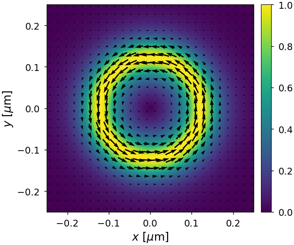
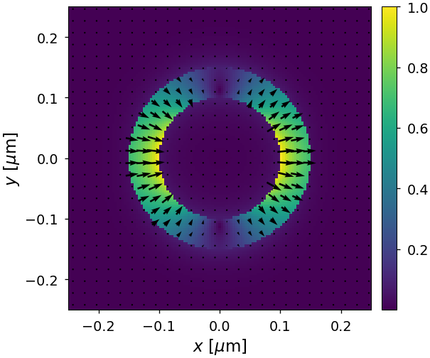
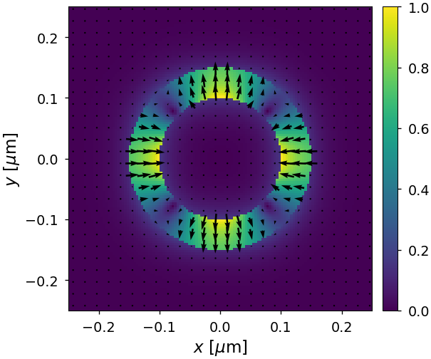
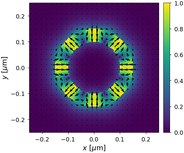
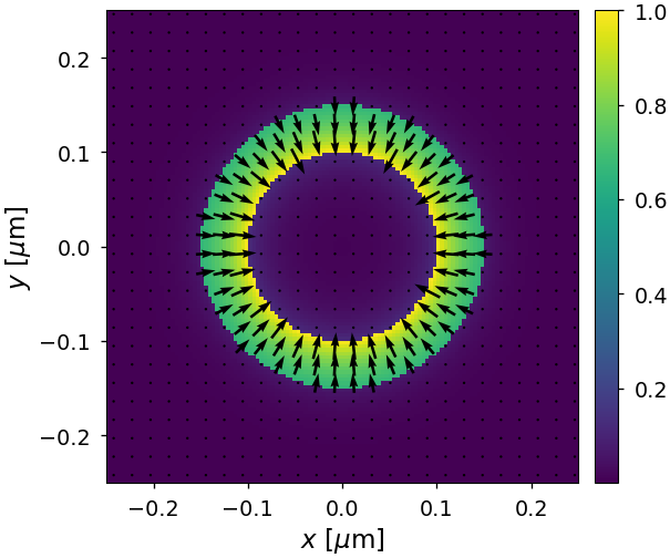
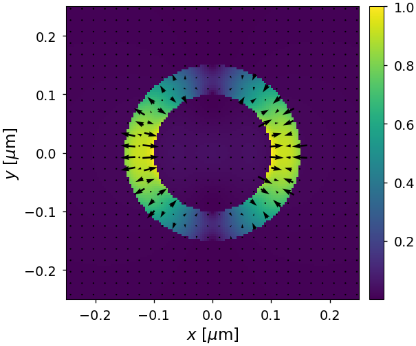
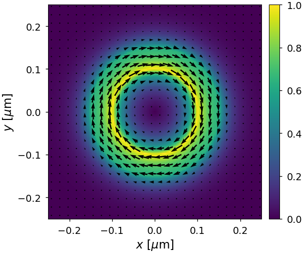
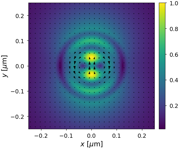
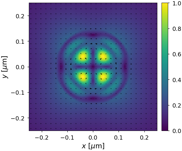
[16]:

wl = 0.6
w = 2 * np.pi / wl
wg1.plot_h_field(w, dir='v', alpha=('E', 0, 1))
wg1.plot_h_field(w, dir='h', alpha=('E', 1, 1))
wg1.plot_h_field(w, dir='h', alpha=('E', 2, 1))
wg1.plot_h_field(w, dir='h', alpha=('E', 3, 1))
wg1.plot_h_field(w, dir='h', alpha=('E', 4, 1))
wg1.plot_h_field(w, dir='h', alpha=('M', 0, 1))
wg1.plot_h_field(w, dir='h', alpha=('M', 1, 1))
wg1.plot_h_field(w, dir='h', alpha=('M', 2, 1))

../_images/notebooks_03_coaxial_waveguide_14_0.png

../_images/notebooks_03_coaxial_waveguide_14_1.png

../_images/notebooks_03_coaxial_waveguide_14_2.png

../_images/notebooks_03_coaxial_waveguide_14_3.png

../_images/notebooks_03_coaxial_waveguide_14_4.png

../_images/notebooks_03_coaxial_waveguide_14_5.png

../_images/notebooks_03_coaxial_waveguide_14_6.png

../_images/notebooks_03_coaxial_waveguide_14_7.png

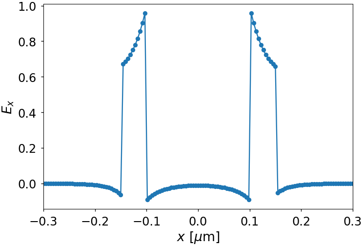
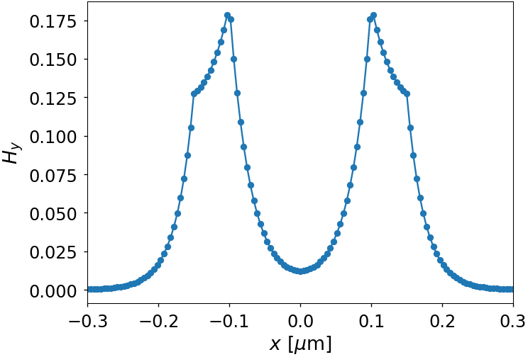
[13]:

wl = 0.6
w = 2 * np.pi / wl
wg1.plot_e_field_on_x_axis(w, dir='h', alpha=('E', 1, 1), comp='x')
wg1.plot_h_field_on_x_axis(w, dir='h', alpha=('E', 1, 1), comp='y')

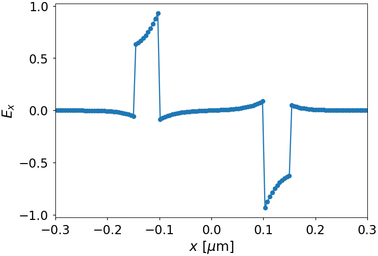
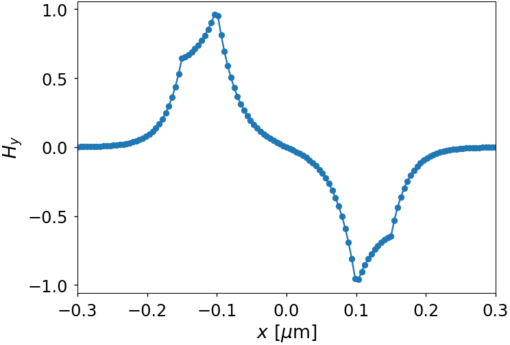
../_images/notebooks_03_coaxial_waveguide_15_0.png

../_images/notebooks_03_coaxial_waveguide_15_1.png

[14]:

wl = 0.6
w = 2 * np.pi / wl
wg1.plot_e_field_on_x_axis(w, dir='h', alpha=('M', 0, 1), comp='x')
wg1.plot_h_field_on_x_axis(w, dir='h', alpha=('M', 0, 1), comp='y')

../_images/notebooks_03_coaxial_waveguide_16_0.png

../_images/notebooks_03_coaxial_waveguide_16_1.png

[ ]: